Function to create weighted data set for competing risks analyses

This function converts a dataset that is in short format (one subject per line) into a counting process format with time-varying weights that correct for right censored and left truncated data. With this data set, analyses based on the subdistribution hazard can be performed.

Usage

# Default S3 method
crprep(
  Tstop,
  status,
  data,
  trans = 1,
  cens = 0,
  Tstart = 0,
  id,
  strata,
  keep,
  shorten = TRUE,
  rm.na = TRUE,
  origin = 0,
  prec.factor = 1000,
  ...
)

Arguments

Tstop: Either 1) a vector containing the time at which the follow-up is ended, or 2) a character string indicating the column name in data that contains the end times (see Details).
status: Either 1) a vector describing status at end of follow-up, having the same length as Tstop, or 2) a character string indicating the column name that contains this information.
data: Data frame in which to interpret Tstart, status, Tstart, id, strata and keep, if given as character value (specification 2, "by name").
trans: Values of status for which weights are to be calculated.
cens: Value that denotes censoring in status column.
Tstart: Either 1) a vector containing the time at which the follow-up is started, having the same length as Tstop, or 2) a character string indicating the column name that contains the entry times, or 3) one numeric value in case it is the same for every subject. Default is 0.
id: Either 1) a vector, having the same length as Tstop, containing the subject identifiers, or 2) a character string indicating the column name containing these subject identifiers. If not provided, a column id is created with subjects having values 1,...,n.
strata: Either 1) a vector of the same length as Tstop, or 2) a character string indicating the column name that contains this information. Weights are calculated for per value in this vector.
keep: Either 1) a data frame or matrix or a numeric or factor vector containing covariate(s) that need to be retained in the output dataset. Number of rows/length should correspond with Tstop, or 2) a character vector containing the column names of these covariates in data.
shorten: Logical. If true, number of rows in output is reduced by collapsing rows within a subject in which weights do not change.
rm.na: Logical. If true, rows for which status is missing are deleted.
origin: Substract origin time units from all Tstop and Tstart times.
prec.factor: Factor by which to multiply the machine's precision. Censoring and truncation times are shifted by prec.factor*precision if event times and censoring/truncation times are equal.
...: Further arguments to be passed to or from other methods. They are ignored in this function.

Value

A data frame in long (counting process) format containing the covariates (replicated per subject). The following column names are used:

Tstart: start dates of dataset
Tstop: stop dates of dataset
status: status of the subject at the end of that row
weight.cens: weights due to censoring mechanism
weight.trunc: weights due to truncation mechanism (if present)
count: row number within subject and event type under consideration
failcode: event type under consideration

The first column is the subject identifier. If the argument "id" is missing, it has values 1:n and is named "id". Otherwise the information is taken from the id argument.

Variables as specified in strata and/or keep are included as well (see Details).

Details

For each event type as specified via trans, individuals with a competing event remain in the risk set with weights that are determined by the product-limit forms of the time-to-censoring and time-to-entry estimates. Typically, their weights change over follow-up, and therefore such individuals are split into several rows. Censoring weights are always computed. Truncation weights are computed only if Tstart is specified.

If several event types are specified at once, regression analyses using the stacked format data set can be performed (see Putter et al. 2007 and Chapter 4 in Geskus 2016). The data set can also be used for a regression on the cause-specific hazard by restricting to the subset subset=count==0.

Missing values are allowed in Tstop, status, Tstart, strata and keep. Rows for which Tstart or Tstart is missing are deleted.

There are two ways to supply the data. If given "by value" (option 1), the actual data vectors are used. If given "by name" (option 2), the column names are specified, which are read from the data set in data. In general, the second option is preferred.

If data are given by value, the following holds for the naming of the columns in the output data set. If keep, strata or id is a vector from a (sub)-list, e.g. obj$name2$name1, then the column name is based on the most inner part (i.e.\ "name1"). If it is a vector of the form obj[,"name1"], then the column is named "name1". For all other vector specifications, the name is copied as is. If keep is a data.frame or a named matrix, the same names are used for the covariate columns in the output data set. If keep is a matrix without names, then the covariate columns are given the names "V1" until "Vk".

The current function does not allow to create a weighted data set in which the censoring and/or truncation mechanisms depend on covariates via a regression model.

References

Geskus RB (2011). Cause-Specific Cumulative Incidence Estimation and the Fine and Gray Model Under Both Left Truncation and Right Censoring. Biometrics 67, 39–49.

Geskus, Ronald B. (2016). Data Analysis with Competing Risks and Intermediate States. CRC Press, Boca Raton.

Putter H, Fiocco M, Geskus RB (2007). Tutorial in biostatistics: Competing risks and multi-state models. Statistics in Medicine 26, 2389–2430.

Author

Ronald Geskus

Examples


data(aidssi)
aidssi.w <- crprep("time", "cause", data=aidssi, trans=c("AIDS","SI"),
                   cens="event-free", id="patnr", keep="ccr5")

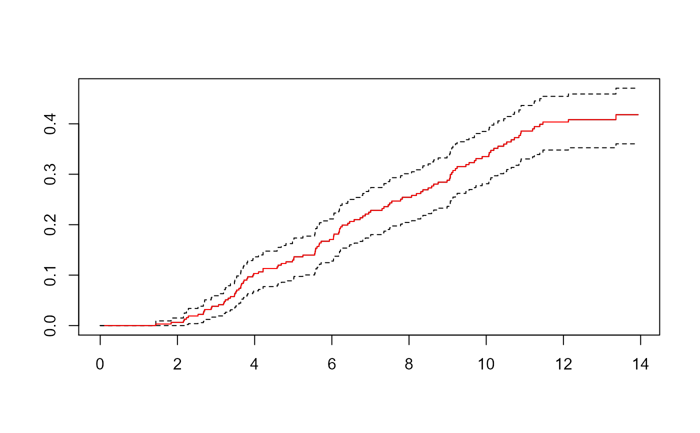
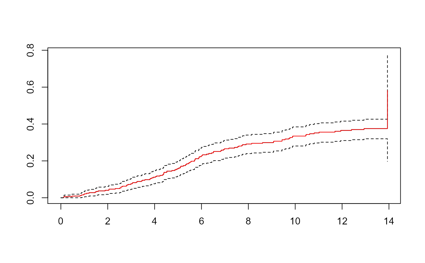
# calculate cause-specific cumulative incidence, no truncation,
# compare with Cuminc (also from mstate)
ci <- Cuminc(aidssi$time, aidssi$status)
sf <- survfit(Surv(Tstart,Tstop,status=="AIDS")~1, data=aidssi.w,
              weight=weight.cens, subset=failcode=="AIDS")
plot(sf, fun="event", mark.time=FALSE)
lines(CI.1~time,data=ci,type="s",col="red")

sf <- survfit(Surv(Tstart,Tstop,status=="SI")~1, data=aidssi.w,
              weight=weight.cens, subset=failcode=="SI")
plot(sf, fun="event", mark.time=FALSE)
lines(CI.2~time,data=ci,type="s",col="red")


# Fine and Gray regression for cause 1
cw <- coxph(Surv(Tstart,Tstop,status=="AIDS")~ccr5, data=aidssi.w,
      weight=weight.cens, subset=failcode=="AIDS")
cw
#> Call:
#> coxph(formula = Surv(Tstart, Tstop, status == "AIDS") ~ ccr5, 
#>     data = aidssi.w, weights = weight.cens, subset = failcode == 
#>         "AIDS")
#> 
#>           coef exp(coef) se(coef) robust se      z        p
#> ccr5WM -1.0041    0.3664   0.3057    0.2819 -3.562 0.000368
#> 
#> Likelihood ratio test=13.95  on 1 df, p=0.0001881
#> n= 7248, number of events= 113 
#>    (43 observations deleted due to missingness)
# This can be checked with the results of crr (cmprsk)
# crr(ftime=aidssi$time, fstatus=aidssi$status, cov1=as.numeric(aidssi$ccr5))

# Gray's log-rank test
aidssi.wCCR <- crprep("time", "cause", data=aidssi, trans=c("AIDS","SI"),
                      cens="event-free", id="patnr", strata="ccr5")
test.AIDS <- coxph(Surv(Tstart,Tstop,status=="AIDS")~ccr5, data=aidssi.wCCR,
                   weights=weight.cens, subset=failcode=="AIDS")
test.SI <- coxph(Surv(Tstart,Tstop,status=="SI")~ccr5, data=aidssi.wCCR,
                 weights=weight.cens, subset=failcode=="SI")
## score test statistic and p-value
c(test.AIDS$score, 1-pchisq(test.AIDS$score,1)) # AIDS
#> [1] 1.296891e+01 3.167068e-04
c(test.SI$score, 1-pchisq(test.SI$score,1))     # SI
#> [1] 0.3941795 0.5301106
# This can be compared with the results of cuminc (cmprsk)
# with(aidssi, cuminc(time, status, group=ccr5)$Tests)
# Note: results are not exactly the same