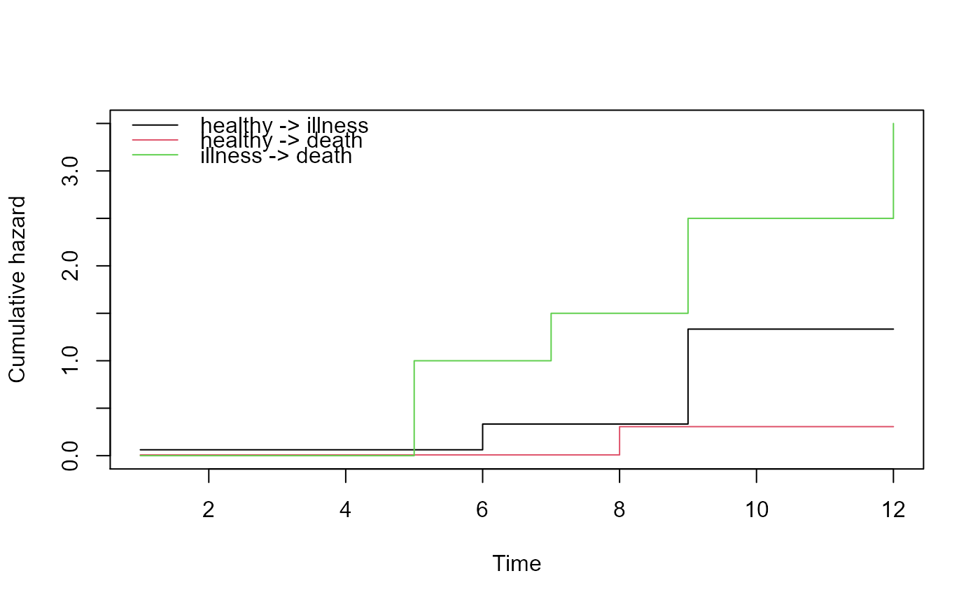
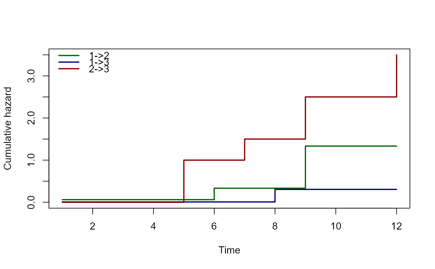
Plot method for an msfit object

Plot method for an object of class "msfit". It plots the estimated cumulative transition intensities in the multi-state model.

Usage

# S3 method for class 'msfit'
plot(
  x,
  type = c("single", "separate"),
  cols,
  xlab = "Time",
  ylab = "Cumulative hazard",
  ylim,
  lwd,
  lty,
  legend,
  legend.pos = "right",
  bty = "n",
  use.ggplot = FALSE,
  xlim,
  scale_type = "fixed",
  conf.int = 0.95,
  conf.type = "none",
  ...
)

Arguments

x

Object of class "msfit", containing estimated cumulative transition intensities for all transitions in a multi-state model

type

One of "single" (default) or "separate"; in case of "single", all estimated cumulative hazards are drawn in a single plot, in case of "separate", separate plots are shown for the estimated transition intensities

cols

A vector specifying colors for the different transitions; default is 1:K (K no of transitions), when type="single", and 1 (black), when type="separate"

xlab

A title for the x-axis; default is "Time"

ylab

A title for the y-axis; default is "Cumulative hazard"

ylim

The y limits of the plot(s); if ylim is specified for type="separate", then all plots use the same ylim for y limits

lwd

The line width, see par; default is 1

lty

The line type, see par; default is 1

legend

Character vector of length equal to the number of transitions, to be used in a legend; if missing, these will be taken from the row- and column-names of the transition matrix contained in x$trans. Also used as titles of plots for type="separate"

legend.pos

The position of the legend, see legend; default is "topleft"

bty

The box type of the legend, see legend

use.ggplot

Default FALSE, set TRUE for ggplot version of plot

xlim

Limits of x axis, relevant if use_ggplot = T

scale_type

"fixed", "free", "free_x" or "free_y", see scales argument of facet_wrap(). Only relevant for use_ggplot = T.

conf.int

Confidence level (%) from 0-1 for the cumulative hazard, default is 0.95. Only relevant for use_ggplot = T

conf.type

Type of confidence interval - either "log" or "plain" . See function details of plot.probtrans for details

...

Further arguments to plot

Value

No return value

See also

msfit

Author

Hein Putter H.Putter@lumc.nl

Edouard F. Bonneville e.f.bonneville@lumc.nl

Examples

# transition matrix for illness-death model
tmat <- trans.illdeath()
# data in wide format, for transition 1 this is dataset E1 of
# Therneau & Grambsch (2000)
tg <- data.frame(illt=c(1,1,6,6,8,9),ills=c(1,0,1,1,0,1),
        dt=c(5,1,9,7,8,12),ds=c(1,1,1,1,1,1),
        x1=c(1,1,1,0,0,0),x2=c(6:1))
# data in long format using msprep
tglong <- msprep(time=c(NA,"illt","dt"),status=c(NA,"ills","ds"),
    data=tg,keep=c("x1","x2"),trans=tmat)
# events
events(tglong)
#> $Frequencies
#>          to
#> from      healthy illness death no event total entering
#>   healthy       0       4     2        0              6
#>   illness       0       0     4        0              4
#>   death         0       0     0        6              6
#> 
#> $Proportions
#>          to
#> from        healthy   illness     death  no event
#>   healthy 0.0000000 0.6666667 0.3333333 0.0000000
#>   illness 0.0000000 0.0000000 1.0000000 0.0000000
#>   death   0.0000000 0.0000000 0.0000000 1.0000000
#> 
table(tglong$status,tglong$to,tglong$from)
#> , ,  = 1
#> 
#>    
#>     2 3
#>   0 2 4
#>   1 4 2
#> 
#> , ,  = 2
#> 
#>    
#>     2 3
#>   0 0 0
#>   1 0 4
#> 
# expanded covariates
tglong <- expand.covs(tglong,c("x1","x2"))
# Cox model with different covariate
cx <- coxph(Surv(Tstart,Tstop,status)~x1.1+x2.2+strata(trans),
  data=tglong,method="breslow")
summary(cx)
#> Call:
#> coxph(formula = Surv(Tstart, Tstop, status) ~ x1.1 + x2.2 + strata(trans), 
#>     data = tglong, method = "breslow")
#> 
#>   n= 16, number of events= 10 
#> 
#>        coef exp(coef) se(coef)     z Pr(>|z|)
#> x1.1 1.4753    4.3723   1.2557 1.175    0.240
#> x2.2 0.8571    2.3563   0.8848 0.969    0.333
#> 
#>      exp(coef) exp(-coef) lower .95 upper .95
#> x1.1     4.372     0.2287    0.3731     51.24
#> x2.2     2.356     0.4244    0.4160     13.35
#> 
#> Concordance= 0.781  (se = 0.077 )
#> Likelihood ratio test= 2.93  on 2 df,   p=0.2
#> Wald test            = 2.32  on 2 df,   p=0.3
#> Score (logrank) test = 2.86  on 2 df,   p=0.2
#> 
# new data, to check whether results are the same for transition 1 as
# those in appendix E.1 of Therneau & Grambsch (2000)
newdata <- data.frame(trans=1:3,x1.1=c(0,0,0),x2.2=c(0,1,0),strata=1:3)
msf <- msfit(cx,newdata,trans=tmat)
# standard plot
plot(msf)

# specifying line width, color, and legend
plot(msf,lwd=2,col=c("darkgreen","darkblue","darkred"),legend=c("1->2","1->3","2->3"))

# separate plots
par(mfrow=c(2,2))
plot(msf,type="separate",lwd=2)
par(mfrow=c(1,1))


# ggplot version - see vignette for details
library(ggplot2)
plot(msf, use.ggplot = TRUE)